
In the previous post in this series I talked about why it’s a good idea to have a hand on your personal finances, now I’m going to show you how to do it in very practical and easy to follow terms. Some of the steps will vary depending on how your bank works.
First things first; you will need to obtain at least three months and preferably 6 months of bank statements for your main bank account. If you have a credit card(s) you should also obtain the statements for those, and if you don’t have a joint account where your salary and your spouses (if you have one) are paid into, then you should also obtain his/her bank statements too. It can get complicated but by breaking it down into individual accounts, it is relatively simple to keep the whole thing under control.
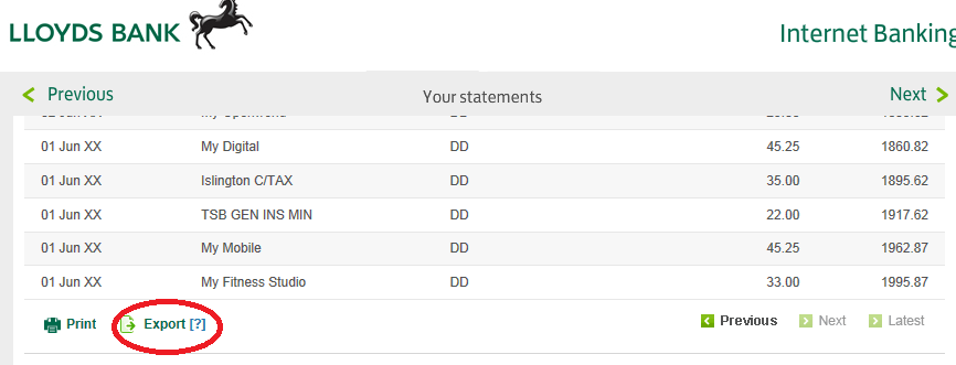
The majority of UK banks, including Lloyds and Barclays to name but two, allow customers who have online banking set up to download their current and previous bank statements. The format you need to choose can be a little confusing- you do not want to pick PDF or anything like that, you need to pick .CSV
CSV, Comma Separated Varible files can be imported into any spreadsheet package. If you have MS Excel installed on your machine, you can simply double click the downloaded CSV to open it. Of course MS Office isn’t free, unless you were lucky enough to have it bundled on your PC when you bought it, so there are other Office suites available like:
- Libre Office
- Open Office
- Google Docs/Drive
If you have a Google account, you’re already able to use Google Docs and for this reason, combined with the fact that it is browser based and you can consequently access it anywhere, my personal choice is Google Docs.
If, for some reason, you cannot get hold of a .CSV file of your bank statements then you’ll have to consider whether it’s possible to cut and paste the details from an onscreen display into a spreadsheet. If it is not, you may have to do it the long handed way, typing in the details from hard copy bank statement.
For the purposes of the rest of this piece, I am going to illustrate the work required using Google Docs.
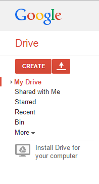
Firstly, navigate to the Google homepage and ensure you are logged in to your account. In the top right of the screen you will see a grid of 9 squares. Click on this and select “Drive”.

This will take you into Google Drive. Now, assuming you have downloaded a CSV file of your transactions, you simply have to hit the upload button and navigate to where your download is situated. The upload icon is the little upward pointing arrow:
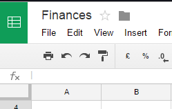
You should now have you statement in as a Google Spreadsheet!
At present all you have is the raw data, with no analysis, which is not a great deal of help to be honest. The first thing to do is to delete any extraneous columns. For the purpose of our cashbook, all we need is the date, transaction type, the narrative on who the payment is made to/from, and the debit and credit (payment & receipt) columns. you can delete every other column. To delete a column, simply right click on the letter at the top of the column and select Delete column from the contextual menu. Don’t worry if you delete the wrong column, there is an undo function on the toolbar- the back arrow next to the print icon:
If you find a column is wide enough to show all the text, hover the mouse pointer between the column in question and the next one. The cursor will change to a double ended arrow- if you right click now it will automatically adjust the column to the width of the widest text.
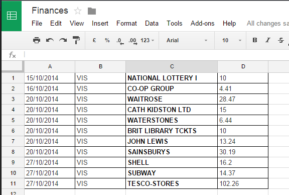
Now your spreadsheet should look something like this:
In itself this is partially useful- you can sort the B column by transaction type to look at your monthly direct debits for example. To do this, highlight all of the cells in your spreadsheet, and then hit the funnel icon:
![]()
This should result in a drop down icon appearing to the top right of each of the cells in the first row. Hitting the drop down will give you certain filter options:
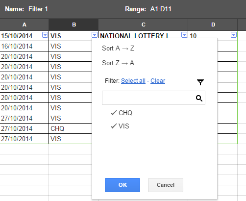
Clearing the filter and selecting, for example, DD for direct debits or SO for standing orders, should allow you to identify any regular monthly outgoings. However, whilst this is useful for an initial examination of what fixed expenditure you have, the real help comes from summarising each of these individual payments into categories that you can then total to see how much you spend on each area every month.
The choice of categories is of course entirely up to you and will vary from person to person. Personally I choose to have the following as column categories:
- Utilities (gas, electric, water, TV license, broadband, landline telephone)
- Mortgage
- Food shopping
- Mobile phones
- Household goods
- Car running costs (fuel, road tax, servicing etc)
- Entertainment
- Other
You can either have less or more, depending on your personal circumstances. There is a fine line between having enough analysis and too much- if you break it down too much you won’t have much actual analysis after all.
In terms of actually putting the numbers into the separate columns, there are several ways to do this. Personally I always like having a total column that you can run a finger down, so I would be tempted to use an easy formula to populate the cells in the category column. Simply highlight the cell and press the “=” (equals) key. then move the cursor left to the cell on the same line with the figure in it and press enter. Hey presto! You have a cell that will total whatever came from your bank statement.
In terms of how much to actually download, as I’v e already said, at the start I would recommend three months as a bare minimum. Anything less and you won’t get a proper picture of irregular spending. The more you can do the better.
Once you have your cashbook drawn up, you will need to sum the columns. In my day job as an accountant I have actually seen people add up columns on spreadsheets with a calculator and type the answer. Suffice to say, you don’t have to do this because any spreadsheet package has a useful SUM function and Google Docs are no different.
![]()
The icon on the right, the sigma symbol, has a number of functions available if you click on it. One of these is SUM, and selecting this allows you to drag the cursor over a section of adjacent cells to give you a total. Once you have done this for one column, you can just hover over the square in the bottom right of a cell and drag the formula across:
![]()
Now you should have the cashbook totalled up and we’re ready to move on to the next stage, which is the interesting one…